Visualizing L1 and L2 Regularization on a Cross-Entropy Loss Surface

I had wanted to write this post for a long time. Once I finally got ECharts working inside my blog, I could finish it properly.

The goal here is simple: make L1 and L2 regularization visible. Instead of discussing them only as formulas, we will look at how they reshape a cross-entropy loss surface in 3D. That makes several abstract ideas much easier to grasp, especially why L1 regularization often produces sparse models and therefore behaves a bit like feature selection.

I first became curious about this after hearing someone describe the “sharp corner” created by L1 regularization. That immediately raised a question for me: what would the full loss surface look like if we plotted it directly? This article is my attempt to answer that question visually.

1. Cross-Entropy Loss ¶

Consider a very small neural network:

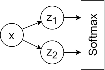
Its forward pass can be written as: $$\hat{z_1}=\beta_1x$$ $$\hat{z_2}=\beta_2x$$ $$Softmax(\hat{z_i}),\ i\in{2}$$

This network has only two parameters, $\beta_1$ and $\beta_2$.

Now consider the cross-entropy loss: $$J(\beta)=-p\log(q)-(1-p)\log(1-q)$$ $$=-p\log(\frac{e^{\beta_1x}}{e^{\beta_1x}+e^{\beta_2x}})-(1-p)\log(\frac{e^{\beta_2x}}{e^{\beta_1x}+e^{\beta_2x}})$$ $$=…$$ $$=-p\log{e^{\beta_1x}}-(1-p)log{e^{\beta_2x}}+log(e^{\beta_1x}+e^{\beta_2x})$$ $$=-p\beta_1x-(1-p)\beta_2x+log(e^{\beta_1x}+e^{\beta_2x})$$

Here, $p$ is the ground-truth probability for class $z_1$, $1-p$ is the probability for class $z_2$, $\beta_1$ and $\beta_2$ are the model parameters, and $x$ is a scalar input.

Using this formula, we can visualize the loss surface directly:

All 3D plots below can be rotated and zoomed.

For simplicity, both $p$ and $x$ are fixed at 1, because the point here is to see how the loss changes as $\beta_1$ and $\beta_2$ move.

The surface is smooth. Its minimum keeps drifting toward the direction where $\beta_1 \to +\infty$ and $\beta_2 \to -\infty$. Intuitively, without regularization, gradient-based optimization keeps rewarding larger and larger parameter magnitudes if that continues to separate the classes better, which is one reason overfitting becomes a concern.

2. Cross-Entropy Loss with L1 Regularization ¶

To prevent parameters from growing too large in magnitude, we can add a regularization term.

With L1 regularization, the loss becomes:

$$J(\beta)=-p\beta_1x-(1-p)\beta_2x+log(e^{\beta_1x}+e^{\beta_2x})+\lambda{(||\beta_1||_1+||\beta_2||_1)}$$

where $\lambda$ is the L1 regularization strength.

The plots below show how different values of $\lambda$ change the shape of the loss surface:

My own first reaction to these plots was that they are both beautiful and surprisingly informative. A 3D surface turns an abstract optimization idea into something you can inspect directly.

The key visual change is that L1 regularization introduces folds into the surface, and the fold becomes sharper as $\lambda$ increases.

More importantly, those folds lie exactly on the lines $\beta_1=0$ and $\beta_2=0$. That makes it easier for optimization to land on parameter values that are exactly zero. And that is the geometric reason L1 regularization tends to produce sparse models.

import tensorflow as tf
x = tf.Variable(0.0)
y = tf.where(tf.greater(x, 0), x+2, 2)  # Piecewise function: y=2 (x<0), y=x+2 (x>=0)
grad = tf.gradients(y, [x])[0]
with tf.Session() as sess:
    sess.run(tf.global_variables_initializer())
    print(sess.run(grad))

3. Cross-Entropy Loss with L2 Regularization ¶

Now let us add L2 regularization:

$$J(\beta)=-p\beta_1x-(1-p)\beta_2x+log(e^{\beta_1x}+e^{\beta_2x})+\Omega{(||\beta_1||_2^2+||\beta_2||_2^2)}$$

The plots below show the loss surface for different values of the L2 coefficient $\Omega$:

L2 regularization changes the surface in a very different way. Instead of creating folds, it bends the surface smoothly. The minimum is no longer pushed toward $\beta_1 \to +\infty$ and $\beta_2 \to -\infty$; it moves to a finite location. As the L2 coefficient grows, that minimum also shifts closer to the origin at $(0, 0)$.

4. Cross-Entropy Loss with Both L1 and L2 Regularization ¶

Of course, L1 and L2 can also be used together:

This combined surface inherits properties from both penalties: the smooth pull of L2 and the axis-aligned folds introduced by L1.

5. Conclusion ¶

L1 regularization:

• Penalizes the sum of absolute values of the parameters, which encourages sparsity
• Often behaves like feature selection because some parameters are driven exactly to zero
• Produces simpler, more interpretable models, though this can make it harder to capture very complex relationships
• Tends to be more robust to outliers

L2 regularization:

• Penalizes the sum of squared parameter values, which encourages smaller but usually nonzero weights
• Produces dense models rather than sparse ones
• Usually preserves more information across features and often leads to better predictive performance
• Is more sensitive to outliers than L1

Further reading:

What does regularization mean in machine learning? (Chinese) https://zhuanlan.zhihu.com/p/62615141